General Theory Of Pipeline

Introduction: The example just completed illustrates the following general theory underlying pipelining: if we can come up with at least two different outermost loops for a loop nest and satisfy all the dependences, then we can pipeline the computation. A loop with k outermost fully permutable loops has k - 1 degrees of pipelined parallelism.

Loops that cannot be pipelined do not have alternative outermost loops. Example 11.56 shows one such instance. To honor all the dependences, each iteration in the outermost loop must execute precisely the computation found in the original code. However, such code may still contain parallelism in the inner loops, which can be exploited by introducing at least n synchronizations, where n is the number of iterations in the outermost loop.

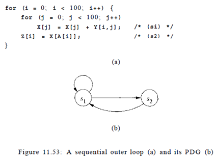
Example: Figure 11.53 is a more complex version of the problem we saw in Example 11.50. As shown in the program dependence graph in Fig. 11.53(b), statements s\ and s2 belong to the same strongly connected component. Because we do not know the contents of matrix A, we must assume that the access in statement s2 may read from any of the elements of X. There is a true dependence from statement si to statement s2 and an anti dependence from statement s2 to statement sx . There is no opportunity for pipelining either, because all operations belonging to iteration i in the outer loop must precede those in iteration i To find more parallelism, we repeat the parallelization process on the inner loop. The iterations in the second loop can be parallelized without synchronization. Thus, 200 barriers are needed, with one before and one after each execution of the inner loop.

Time-Partition Constraints: We now focus on the problem of finding pipelined parallelism. Our goal is to turn a computation into a set of pipelinable tasks. To find pipelined parallelism, we do not solve directly for what is to be executed on each processor, like we did with loop parallelization. Instead, we ask the following fundamental question:

What are all the possible execution sequences that honor the original data dependences in the loop? Obviously the original execution sequence satisfies all the data dependences. The question is if there are affine transformations that can create an alternative schedule, where iterations of the outermost loop execute a different set of operations from the original, and yet all the dependences are satisfied. If we can find such transforms, we can pipeline the loop. The key point is that if there is freedom in scheduling operations, there is parallelism; details of how we derive pipelined parallelism from such transforms will be explained later. To find acceptable re-orderings of the outer loop, we wish to find one-dimensional affine transforms, one for each statement, that map the original loop index values to an iteration number in the outermost loop. The transforms are legal if the assignment can satisfy all the data dependences in the program. The "time-partition constraints," shown below, simply say that if one operation is dependent upon the other, then the first must be assigned an iteration in the outermost loop no earlier than that of the second. If they are assigned in the same iteration, then it is understood that the first will be executed after than the second within the iteration.

An affine-partition mapping of a program is a legal-time partition if and only if for every two (not necessarily distinct) accesses sharing dependence, say

Fi = < F i , f i , B i , b i)

in statement s\, which is nested in d\ loops, and

T2 = ( F 2 , f 2 , B 2 , b 2)

in statement s2 nested in d2 loops, the one-dimensional partition mappings ( C i , c i ) and ( C 2 , c 2 ) for statements si and s2 , respectively, satisfy the time partition constraints:

For all ii in Zdl and i2 in Zd* such that

a)      a ) ii - < S l s 2 h,

b)      Biii b i > 0,

c)       B 2 i 2 b2 > 0, and

d)      F i i i fi = F 2 i 2 f2,

it is the case that C i i i ci < C 2 i 2 c 2 .

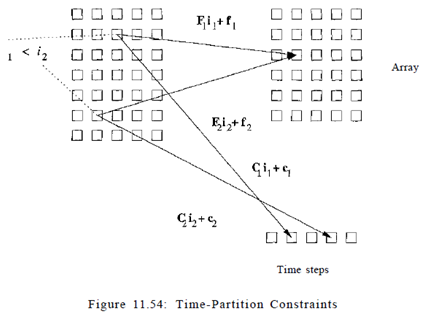
This constraint, illustrated in Fig. 11.54, looks remarkably similar to the space-partition constraints. It is a relaxation of the space-partition constraints, in that if two iterations refer to the same location, they do not necessarily have to be mapped to the same partition; we only require that the original relative execution order between the two iterations is preserved. That is, the constraints here have < where the space-partition constraints have.

We know that there exists at least one solution to the time-partition constraints. We can map operations in each iteration of the outermost loop back to the same iteration, and all the data dependences will be satisfied. This solution is the only solution to the time-partition constraints for programs that cannot be pipelined. On the other hand, if we can find several independent solutions to time-partition constraints, the program can be pipelined. Each independent solution corresponds to a loop in the outermost fully permutable nest. As you can expect, there is only one independent solution to the timing constraints extracted from the program, where there is no pipelined parallelism, and that there are two independent solutions to the SOR code example