Support Vector Machines

Introduction: In a nutshell, a support vector machine (or SVM) is an algorithm that works as follows. It uses a nonlinear mapping to transform the original training data into a higher dimension. Within this new dimension, it searches for the linear optimal separating hyper plane (that is, a “decision boundary” separating the tuples of one class from another). With an appropriate nonlinear mapping to a sufficiently high dimension, data from two classes can always be separated by a hyper plane. The SVM finds this hyper plane using support vectors (“essential” training tuples) and margins (defined by the support vectors).We will delve more into these new concepts further below.

“I’ve heard that SVMs have attracted a great deal of attention lately. Why?” The first paper on support vector machines was presented in 1992 by Vladimir Vapnik and colleagues Bernhard Boser and Isabelle Guyon, although the groundwork for SVMs has been around since the 1960s (including early work by Vapnik and Alexei Chervonenk is on statistical learning theory). Although the training time of even the fastest SVMs can be extremely slow, they are highly accurate, owing to their ability to model complex nonlinear decision boundaries. They are much less prone to over fitting than other methods. The support vectors found also provide a compact description of the learned model. SVMs can be used for prediction as well as classification. They have been applied to a number of areas, including handwritten digit recognition, object recognition, and speaker identification, as well as benchmark time-series prediction tests.

The Case When the Data Are Linearly Separable

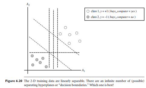
To explain the mystery of SVMs, let’s first look at the simplest case a two-class problem where the classes are linearly separable. Let the data set D be given as (X1, y1), (X2, y2), : : : , (X|D|, y_|D|),where Xi is the set of training tuples with associated class labels, yi. Each yi can take one of two values, either 1 or-1 (i.e., yi ∈ { 1, -1}), corresponding to the classes buys computer = yes and buys computer = no, respectively. To aid in visualization, let’s consider an example based on two input attributes, A1 and A2, as shown in Figure 6.20. From the graph, we see that the 2-D data are linearly separable (or “linear,” for short) because a straight line can be drawn to separate all of the tuples of class 1 from all of the tuples of class-1. There are an infinite number of separating lines that could be drawn. We want to find the “best” one, that is, one that (we hope) will have the minimum classification error on previously unseen tuples. How can we find this best line? Note that if our data were 3-D (i.e., with three attributes), we would want to find the best separating plane. Generalizing to n dimensions, we want to find the best hyper plane. We will use the term “hyper plane” to refer to the decision boundary that we are seeking, regardless of the number of input attributes. So, in other words, how can we find the best hyper plane?

An SVM approaches this problem by searching for the maximum marginal hyper plane. Consider Figure 6.21, which shows two possible separating hyper planes and their associated margins. Before we get into the definition of margins, let’s take an intuitive look at this figure. Both hyper planes can correctly classify all of the given data tuples. Intuitively, however, we expect the hyper plane with the larger margin to be more accurate at classifying future data tuples than the hyper plane with the smaller margin. This is why (during the learning or training phase), the SVM searches for the hyper plane with the largest margin, that is, the maximum marginal hyper plane (MMH). The associated margin gives the largest separation between classes. Getting to an informal definition of margin, we can say that the shortest distance from a hyper plane to one side of its margin is equal to the shortest distance from the hyper plane to the other side of its margin, where the “sides” of the margin are parallel to the hyper plane. When dealing with the MMH, this distance is, in fact, the shortest distance from the MMH to the closest training tuple of either class.

A separating hyper plane can be written as

W.X b = 0;