Basic Operations On B-trees

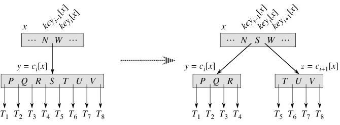
		B-TREE-SPLIT-CHILD(x, i, y)
 1  z ← ALLOCATE-NODE()
 2  leaf[z] ← leaf[y]
 3  n[z] ← t - 1
 4  for j ← 1 to t - 1
 5       do keyj[z] ← keyj t[y]
 6  if not leaf [y]
 7     then for j ← 1 to t
 8              do cj[z] ← cj t[y]
 9  n[y] ← t - 1
10  for j ← n[x]   1 downto i   1
11       do cj 1[x] ← cj [x]
12  ci 1[x] ← z
13  for j ← n[x] downto i
14       do keyj 1[x] ← keyj[x]
15  keyi[x] ← keyt[y]
16  n[x] ← n[x]   1
17  DISK-WRITE(y)
18  DISK-WRITE(z)
19  DISK-WRITE(x)

B-TREE-SPLIT-CHILD works by straightforward "cutting and pasting." Here, y is the ith child of x and is the node being split. Node y originally has 2t children (2t - 1 keys) but is reduced to t children (t - 1 keys) by this operation. Node z "adopts" the t largest children (t - 1 keys) of y, and z becomes a new child of x, positioned just after y in x's table of children. The median key of y moves up to become the key in x that separates y and z.

Lines 1-8 create node z and give it the larger t - 1 keys and corresponding t children of y. Line 9 adjusts the key count for y. Finally, lines 10-16 insert z as a child of x, move the median key from y up to x in order to separate y from z, and adjust x's key count. Lines 17-19 write out all modified disk pages. The CPU time used by B-TREE-SPLIT-CHILD is Θ(t), due to the loops on lines 4-5 and 7-8. (The other loops run for O(t) iterations.) The procedure performs O(1) disk operations.

Inserting a key into a B-tree in a single pass down the tree

We insert a key k into a B-tree T of height h in a single pass down the tree, requiring O(h) disk accesses. The CPU time required is O(th) = O(t log_t n). The B-TREE-INSERT procedure uses B-TREE-SPLIT-CHILD to guarantee that the recursion never descends to a full node.

		B-TREE-INSERT(T, k)
 1  r ← root[T]
 2  if n[r] = 2t - 1
 3     then s ← ALLOCATE-NODE()
 4         root[T] ← s
 5         leaf[s] ← FALSE
 6         n[s] ← 0
 7         c1[s] ← r
 8         B-TREE-SPLIT-CHILD(s, 1, r)
 9         B-TREE-INSERT-NONFULL(s, k)
10    else B-TREE-INSERT-NONFULL(r, k)

Lines 3-9 handle the case in which the root node r is full: the root is split and a new node s (having two children) becomes the root. Splitting the root is the only way to increase the height of a B-tree. Figure 18.6 illustrates this case. Unlike a binary search tree, a B-tree increases in height at the top instead of at the bottom. The procedure finishes by calling B-TREE-INSERT-NONFULL to perform the insertion of key k in the tree rooted at the nonfull root node. B-TREE-INSERT-NONFULL recurses as necessary down the tree, at all times guaranteeing that the node to which it recurses is not full by calling B-TREE-SPLIT-CHILD as necessary.