Bucket Sort
for i = 0, 1, . . ., n - 1. It is no surprise that each bucket i has the same value of  , since each value in the input array A is equally likely to fall in any bucket. To prove equation (8.2), we define indicator random variables
Xij = I{A[j] falls in bucket i}
for i = 0, 1, . . ., n - 1 and j = 1, 2, . . ., n. Thus,

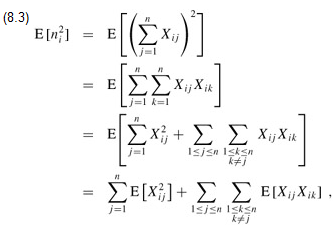
To compute  , we expand the square and regroup terms:

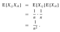
where the last line follows by linearity of expectation. We evaluate the two summations separately. Indicator random variable Xij is 1 with probability 1/n and 0 otherwise, and therefore

When k ≠ j, the variables Xij and Xik are independent, and hence

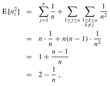
Substituting these two expected values in equation (8.3), we obtain

which proves equation (8.2).
Using this expected value in equation (8.1), we conclude that the expected time for bucket sort is Θ(n) n · O(2 - 1/n) = Θ(n). Thus, the entire bucket sort algorithm runs in linear expected time.
Even if the input is not drawn from a uniform distribution, bucket sort may still run in linear time. As long as the input has the property that the sum of the squares of the bucket sizes is linear in the total number of elements, equation (8.1) tells us that bucket sort will run in linear time.