Counting Sort

Counting sort assumes that each of the n input elements is an integer in the range 0 to k, for some integer k. When k = O(n), the sort runs in Θ(n) time.

The basic idea of counting sort is to determine, for each input element x, the number of elements less than x. This information can be used to place element x directly into its position in the output array. For example, if there are 17 elements less than x, then x belongs in output position 18. This scheme must be modified slightly to handle the situation in which several elements have the same value, since we don't want to put them all in the same position.

In the code for counting sort, we assume that the input is an array A[1 ‥ n], and thus length[A] = n. We require two other arrays: the array B[1 ‥n] holds the sorted output, and the array C[0 ‥ k] provides temporary working storage.

	COUNTING-SORT(A, B, k)
 1  for i ← 0 to k
 2     do C[i] ← 0
 3  for j ← 1 to length[A]
 4     do C[A[j]] ← C[A[j]]   1
 5  ▹ C[i] now contains the number of elements equal to i.
 6  for i ← 1 to k
 7     do C[i] ← C[i]   C[i - 1]
 8  ▹ C[i] now contains the number of elements less than or equal to i.
 9  for j ← length[A] downto 1
10     do B[C[A[j]]] ← A[j]
11        C[A[j]] ← C[A[j]] - 1

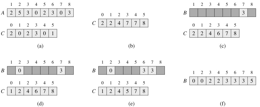
Figure 8.2 illustrates counting sort. After the initialization in the for loop of lines 1-2, we inspect each input element in the for loop of lines 3-4. If the value of an input element is i, we increment C[i]. Thus, after line 4, C[i] holds the number of input elements equal to i for each integer i = 0, 1, . . .,k. In lines 6-7, we determine for each i = 0, 1, . . .,k, how many input elements are less than or equal to i by keeping a running sum of the array C.

Finally, in the for loop of lines 9-11, we place each element A[j] in its correct sorted position in the output array B. If all n elements are distinct, then when we first enter line 9, for each A[j], the value C[A[j]] is the correct final position of A[j] in the output array, since there are C[A[j]] elements less than or equal to A[j]. Because the elements might not be distinct, we decrement C[A[j]] each time we place a value A[j] into the B array. Decrementing C[A[j]] causes the next input element with a value equal to A[j], if one exists, to go to the position immediately before A[j] in the output array.

How much time does counting sort require? The for loop of lines 1-2 takes time Θ(k), the for loop of lines 3-4 takes time Θ(n), the for loop of lines 6-7 takes time Θ(k), and the for loop of lines 9-11 takes time Θ(n). Thus, the overall time is Θ(k n). In practice, we usually use counting sort when we have k = O(n), in which case the running time is Θ(n).

Counting sort beats the lower bound of Ω(n lg n) proved in lower bounds for sorting because it is not a comparison sort. In fact, no comparisons between input elements occur anywhere in the code. Instead, counting sort uses the actual values of the elements to index into an array. The Θ(n lg n) lower bound for sorting does not apply when we depart from the comparison-sort model.

An important property of counting sort is that it is stable: numbers with the same value appear in the output array in the same order as they do in the input array. That is, ties between two numbers are broken by the rule that whichever number appears first in the input array appears first in the output array. Normally, the property of stability is important only when satellite data are carried around with the element being sorted. Counting sort's stability is important for another reason: counting sort is often used as a subroutine in radix sort.