Description Of Quicksort
Description of quicksort: Quicksort, like merge sort, is based on the divide-and-conquer. Here is the three-step divide-and-conquer process for sorting a typical subarray A[p ‥r].
- Divide:Partition (rearrange) the array A[p ‥r] into two (possibly empty) subarrays A[p ‥q - 1] and A[q 1 ‥r] such that each element of A[p ‥q - 1] is less than or equal to A[q], which is, in turn, less than or equal to each element of A[q 1 ‥r]. Compute the index q as part of this partitioning procedure.
- Conquer:Sort the two subarrays A[p ‥q -1] and A[q 1 ‥r] by recursive calls to quicksort.
- Combine:Since the subarrays are sorted in place, no work is needed to combine them: the entire array A[p ‥r] is now sorted.
The following procedure implements quicksort.
QUICKSORT(A, p, r)
1 if p < r
2 then q ← PARTITION(A, p, r)
3 QUICKSORT(A, p, q - 1)
4 QUICKSORT(A, q 1, r)
To sort an entire array A, the initial call is QUICKSORT(A, 1, length[A]).
Partitioning the array: The key to the algorithm is the PARTITION procedure, which rearranges the subarray A[p ‥r] in place.
PARTITION(A, p, r)
1 x ← A[r]
2 i ← p - 1
3 for j ← p to r - 1
4 do if A[j] ≤ x
5 then i ← i 1
6 exchange A[i] ↔ A[j]
7 exchange A[i 1] ↔ A[r]
8 return i 1
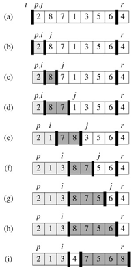
Figure 7.1shows the operation of PARTITION on an 8-element array. PARTITION always selects an element x = A[r] as a pivot element around which to partition the subarray A[p ‥r]. As the procedure runs, the array is partitioned into four (possibly empty) regions. At the start of each iteration of the for loop in lines 3-6, each region satisfies certain properties, which we can state as a loop invariant:

Figure 7.1: The operation of PARTITION on a sample array. Lightly shaded array elements are all in the first partition with values no greater than x. Heavily shaded elements are in the second partition with values greater than x. The unshaded elements have not yet been put in one of the first two partitions, and the final white element is the pivot. (a) The initial array and variable settings. None of the elements have been placed in either of the first two partitions. (b) The value 2 is "swapped with itself" and put in the partition of smaller values. (c)-(d) The values 8 and 7 are added to the partition of larger values. (e) The values 1 and 8 are swapped, and the smaller partition Grows. (f) The values 3 and 8 are swapped, and the smaller partition grows. (g)-(h) The larger partition grows to include 5 and 6 and the loop terminates. (i) In lines 7-8, the pivot element is swapped so that it lies between the two partitions.
-
At the beginning of each iteration of the loop of lines 3-6, for any array index k,
- If p ≤ k ≤ i, then A[k] ≤ x.
- If i 1 ≤ k ≤ j - 1, then A[k] > x.
- If k = r, then A[k] = x.
Figure 7.2summarizes this structure. The indices between j and r - 1 are not covered by any of the three cases, and the values in these entries have no particular relationship to the pivot x.

Figure 7.2: The four regions maintained by the procedure PARTITION on a subarray A[p ‥r]. The values in A[p ‥i] are all less than or equal to x, the values in A[i 1 ‥j - 1] are all greater than x, and A[r] = x. The values in A[j ‥r- 1] can take on any values.