Initial Configuration Of A Multilayer Perceptron

Number of layers: Two or three may often do the job, but more are also used

A network should have one layer of input neurons and one layer of output neurons, which results in at least two layers. During the examination of linear separability at least one hidden layer of neurons, if our problem is not linearly separable (which is, as we have seen, very likely).It is possible, to mathematically prove that this MLP with one hidden neuron layer is already capable of approximating arbitrary functions with any accuracy but it is necessary not only to discuss the representability of a problem by means of a perceptron but also the learnability. Representability means that a perceptron can, in principle, realize a mapping - but learnability means that we are also able to teach it. In this respect, experience shows that two hidden neuron layers (or three trainable weight layers) can be very useful to solve a problem, since many problems can be represented by a hidden layer but are very difficult to learn. One should keep in mind that any additional layer generates additional sub minima of the error function in which we can get stuck. All these things considered, a promising way is to try it with one hidden layer at first and if that fails, retry with two layers. Only if that fails, one should consider more layers. However, given the increasing calculation power of current computers, deep networks with a lot of layers are also used with success.

The number of neurons has to be tested

The number of neurons (apart from input and output layer, where the number of input and output neurons is already defined by the problem statement) principally corresponds to the number of free parameters of the problem to be represented. Since we have already discussed the network capacity with respect to memorizing or a too imprecise problem representation, it is clear that our goal is to have as few free parameters as possible but as many as necessary. But we also know that there is no standard solution for the question of how many neurons should be used. Thus, the most useful approach is to initially train with only a few neurons and to repeatedly train new networks with more neurons until the result significantly improves and, particularly, the generalization performance is not affected (bottom-up approach).

Selecting an activation function

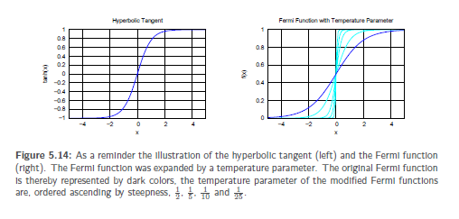
Another very important parameter for the way of information processing of a neural network is the selection of an activation function. The activation function for input neurons is fixed to the identity function, since they do not process information. The first question to be asked is whether we actually want to use the same activation function in the hidden layer and in the output layer – no one prevents us from choosing different functions. Generally, the activation function is the same for all hidden neurons as well as for the output neurons respectively. For tasks of function approximation it has been found reasonable to use the hyperbolic tangent   as activation function of the hidden neurons, while a linear activation function is used in the output. The latter is absolutely necessary so that we do not generate a limited output interval. Contrary to the input layer which uses linear activation functions as well, the output layer still processes information, because it has threshold values. However, linear activation functions in the output can also cause huge learning steps and jumping over good minima in the error surface. This can be avoided by setting the learning rate to very small values in the output layer. An unlimited output interval is not essential for pattern recognition tasks. If the hyperbolic tangent is used in any case, the output interval will be a bit larger. Unlike with the hyperbolic tangent, with the Fermi function it is difficult to learn something far from the threshold value (where its result is close to 0).

Weights should be initialized with small, randomly chosen values

The initialization of weights is not as trivial as one might think. If they are simply initialized with 0, there will be no change in weights at all. If they are all initialized by the same value, they will all change equally during training. The simple solution of this problem is called symmetry breaking, which is the initialization of weights with small random values. The range of random values could be the interval [−0.5; 0.5] not including 0 or values very close to 0. This random initialization has a nice side effect: Chances are that the average of network inputs is close to 0,a value that hits (in most activation functions)the region of the greatest derivative, allowing for strong learning impulses right from the start of learning.