Discrete Probability Spaces
Discrete probability spaces:
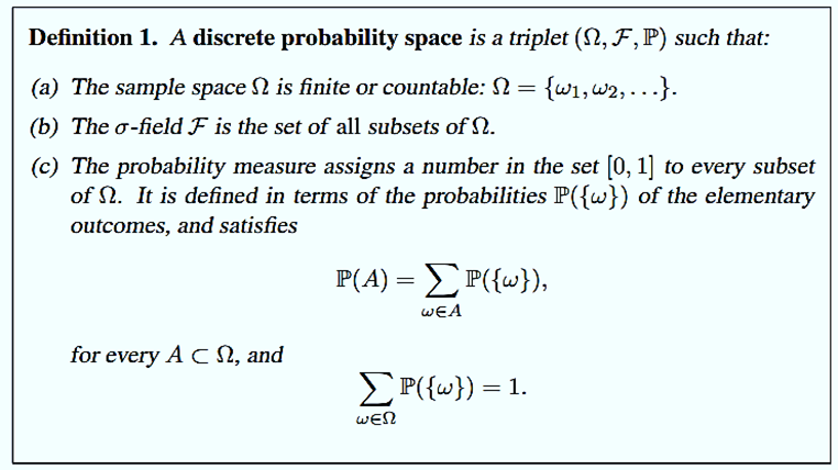
Before continuing with the discussion of σ-fields and probability measures in their full generality, it is helpful to consider the simpler case where the sample space Ω is finite or countable.

For simplicity, we will usually employ the notation P(ω) instead of P({ω}), and we will often denote P(ωi ) by pi
The following are some examples of discrete probability spaces. Note that typically we do not provide an explicit expression for P(A) for every A ⊂Ω. It suffices to specify the probability of elementary outcomes, from which P(A) is readily obtained for any A.
Examples:
(a) Consider a single toss of a coin. If we believe that heads (H) and tails (T) are equally likely, the following is an appropriate model. We set Ω = {ω1, ω2), where ω1 = H and ω2 = T, and let p1 = p2 = 1/2. Here, F = {Ø, {H}, {T}, {H, T}}, and P(Ø) = 0, P(H) = P(T) = 1/2, P({H, T}) = 1.
(b) Consider a single roll of a die. If we believe that all six outcomes are equally likely, the following is an appropriate model. We set Ω = {1, 2 . . . 6} and p1 = · · · = p6 = 1/6.
σ-FIELD:
1. When the sample space Ω is uncountable, the idea of defining the probability of a general subset of Ω in terms of the probabilities of elementary outcomes runs into difficulties.
2. Suppose, for example, that the experiment consists of drawing a number from the interval [0, 1], and that we wish to model a situation where all elementary outcomes are “equally likely.” If we were to assign a probability of zero to every ω, this alone would not be of much help in determining the probability of a subset such as [1/2, 3/4].
3. If we were to assign the same positive value to every ω, we would obtain P({1, 1/2, 1/3, . . .}) = ∞, which is undesirable.
4. A way out of this difficulty is to work directly with the probabilities of more general subsets of Ω (not just subsets consisting of a single element).