Poisson Distribution As A Limit Of The Binomial

Notation:

 Let  us  use  the  abbreviations  dU(a, b),  Ber(p),  Bin(n, p),  Geo(p),  Pois(λ),  and  Pow(α) to  refer  the  above  defined  PMFs.  We  will  use  notation d such  as  X = dU(a, b) or  X ∼dU(a, b) as  a  shorthand  for  the  statement  that  X is  a  discrete  random  variable  whose  PMF  is  uniform  on  (a, b),  and  similarly  for  the  other  PMFs  we  definedY to indicate that  two  random  variables  have  the  same  PMFs.

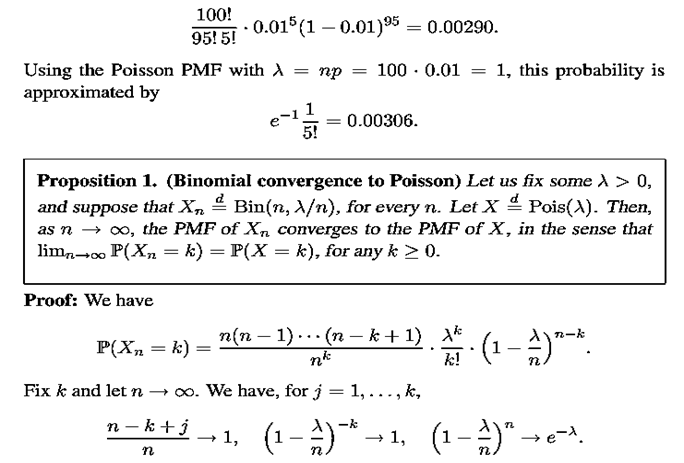
Poisson distribution as a limit of the binomial: To  get  a  feel  for  the  Poisson  random  variable,  think  of  a  binomial  random  vari­able  with  very  small  p and  very  large  n.  For  example,  consider  the  number  of typos  in  a  book  with  a  total  of  n words,  when  the  probability  p that  any  one word is  misspelled is very  small  (associate a word  with a  coin  toss  that  results in a head when the word is  misspelled), or the  number of  cars involved in  accidents in  a  city  on  a  given  day  (associate  a  car  with  a  coin  toss  that  results  in  a  head when the  car has an  accident).  Such random variables can be well modeled with a Poisson PMF. More  precisely,  the  Poisson  PMF  with  parameter  λ is  a  good  approximation for  a  binomial  PMF  with  parameters  n and  p,  i.e.,

provided  λ = np,  n is  large,  and  p is  small.  In  this  case,  using  the  Poisson PMF  may  result  in  simpler  models  and  calculations.  For example, let n = 100and p = 0.01.  Then  the  probability  of  k = 5 successes  in  n = 100 trials  is calculated  using  the  binomial  PMF  as