X-bar And R-charting
Introduction:
Xbar & R charting creates two charts based on continuous quality characteristic values. A fifth, the relatively advanced “Hoteling’s T” method, is described in Chapter 8 and permits simultaneous monitoring of several continuous quality characteristics on a single chart.
Continuous Data: Xbar & R Charting
I. Whenever one or two continuous variable key output variables (KOVs) summarize the quality of units or a system, it is advisable to use a variables charting approach. This follows because variables charting approaches such as Xbar & R charting,
II. These approaches compare favorably in many ways to the attribute charting methods such as p-charting and demerit charting. it will be clear that Xbar & R charts are often based on samples sizes of n = 5 units inspected, compared with 50 or 100 for the attribute charting methods. For a single continuous quality characteristic, Xbar & R charting involves the generation of two charts with two sets of control limits.
III. Two continuous characteristics would require four charts. Generally, when monitoring any more than two continuous quality characteristics, most experts would recommend a multivariate charting method such as the “Hotelling’s T2” charting;
IV. There is no universal standard rule for selecting the number of samples to be included in rational subgroups for Xbar & R charting.
V. Generally, one considers first inspecting only a small fraction of the units, such as 5 out of 200. However, Xbar & R charting could conceivably have application even if complete inspection of all units is completed.
VI. Two considerations for sample size selection follow:
a) First, the larger the sample size, the closer the control limits and the more sensitive the chart will be to assignable causes. Before constructing the charts, however, there is usually no way to know how close the limits will be. Therefore, an iterative process could conceivably be applied. If the limits are too wide, the sample size could be increased and a new chart could be generated.
b) Second, n should ideally be large enough that the sample averages of the value follow a specific pattern. The pattern in question relates to the so-called “normal” distribution. In many situations, this pattern happens automatically if n =4. This common fact explains why practitioners rarely check whether n is large enough such that the sample averages are approximately normally distributed.
Algorithm Standard Xbar & R charting:
Step 1.(Startup) Measure the continuous characteristics, Xi,j, for i = 1,…,n units for j = 1,…,25 periods. Each n units is carefully chosen to be representative of all units in that period, i.e., a rational subgroup.
Step 2.(Startup) Calculate the sample averages Xbar,j = (X1,j … Xn,j)/n and ranges Rj = Max[X1,j,…, Xn,j] – Min[X1,j,…, Xn,j] for j = 1,…,25. Also, calculate the average of all of the 25n numbers, Xbarbar, and the average of the 25 ranges Rbar = (R1 … R25)/25.
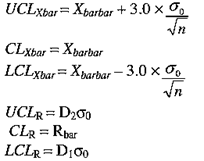
Step 3.(Startup) Tentatively determine σ0 using σ0 = Rbar/d2, where d2 comes from the following table. Use linear interpolation to find d2 if necessary. Calculate the “trial” control limits using

where D1 and D2 also come from Table and where the “trial” designation has been omitted to keep the notation readable.
Step 4.(Startup) Find all the periods for which either Xbar,j or Rj or both are not inside their control limits, i.e., {Xbar,j < LCLXbar or Xbar,j > UCLXbar} and/or {Rj < LCLR or Rj > UCLR}. If the results from any of these periods are
believed to be not representative of future system operations, e.g., because problems were fixed permanently, remove the data from the l not representative periods from consideration.
Step 5.(Startup) Re-calculate Xbar bar and Rbar based on the remaining 25 – l periods and (25 – l) × n data. Also, calculate the revised process sigma, σ0,using σ0 = Rbar/d2. The quantity 6σ0 is called the “process capability” in thecontext of Xbar & R charting. It constitutes a typical range of the qualitycharacteristics. Calculate the revised limits using the same “trial” equationsin Step 3.