Hysteresis Loss:

Unidirectional time varying exciting current: Consider a magnetic circuit with constant (d.c) excitation current I₀. Flux established will have fixed value with a fixed direction. Suppose this final current I₀ has been attained from zero current slowly by energizing the coil from a potential divider arrangement as depicted in Figure (A). Let us also assume that initially the core was not magnetized. The exciting current therefore becomes a function of time till it reached the desired current I and we stopped further increasing it. The flux too naturally will be function of time and cause induced voltage e₁₂ in the coil with a polarity to oppose the increase of inflow of current as shown. The coil becomes a source of emf with terminal-1, ve and terminal-2, -ve. Recall that a source in which current enters through its ve terminal absorbs power or energy while it delivers power or energy when current comes out of the ve terminal. Therefore during the interval when i(t) is increasing the coil absorbs energy. Is it possible to know how much energy does the coil absorb when current is increased from 0 to I₀? This is possible if we have the B-H curve of the material with us.

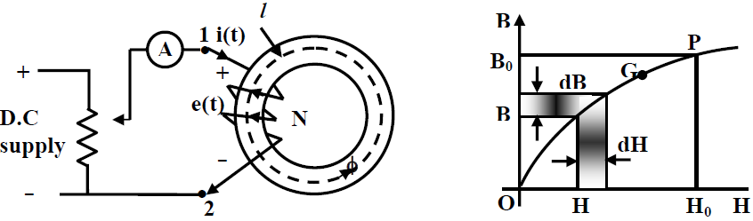fig(A)

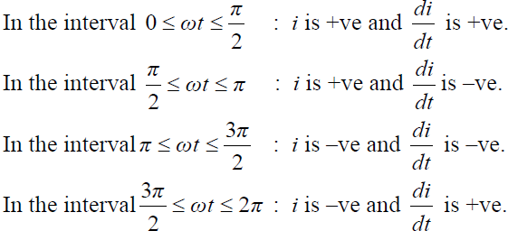
Hysteresis loop with alternating exciting current: In the light of the above discussion, let us see how the operating point is traced out if the exciting current is  i = I_max sin ωt. The nature of the current variation in a complete cycle can be enumerated as follows:

Let the core had no residual field when the coil is excited by i = I_max sin ωt. In the interval 0<ωt<π/2,  B will rise along the path OGP. Operating point at P corresponds to I_max or H_max. For the interval π/2<ωt<π operating moves along the path PRT. At point T, current is zero. However, due to sinusoidal current, i starts increasing in the –ve direction as shown in the Figure 22.10 and operating point moves along TSEQ. It may be noted that a –ve H of value OS is necessary to bring the residual field to zero at S. OS is called the coercivity of the material. At the end of the interval π<ωt<3π/2 current reaches –Imax or field –Hmax. In the next internal, 3π/2π<ωt<2π, current changes from –I_max to zero and operating point moves from M to N along the path MN. After this a new cycle of current variation begins and the operating point now never enters into the path OGP. The movement of the operating point can be described by two paths namely: (i) QFMNKP for increasing current from –I_max to I_max and (ii) from I_max to –I_max along PRTSEQ.

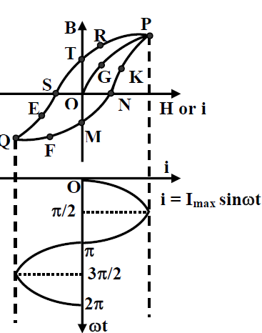fig.(A)