Mining Quantitative Association Rules
Introduction: Quantitative association rules are multidimensional association rules in which the numeric attributes are dynamically discretized during the mining process so as to satisfy some mining criteria, such as maximizing the confidence or compactness of the rules mined. In this section, we focus specifically on how to mine quantitative association rules having two quantitative attributes on the left-hand side of the rule and one categorical attribute on the right-hand side of the rule. That is,
Aquan1 ^Aquan2 ->Acat
where Aquan1 and Aquan2 are tests on quantitative attribute intervals (where the intervals are dynamically determined), and A cat tests a categorical attribute from the task-relevant data. Such rules have been referred to as two-dimensional quantitative association rules, because they contain two quantitative dimensions. For instance, suppose you are curious about the association relationship between pairs of quantitative attributes, like customer age and income, and the type of television (such as high-definition TV, i.e., HDTV) that customers like to buy. An example of such a 2-D quantitative association rule is
age(X, “30:::39”) ^ income(X, “42K…..48K”))buys(X, “HDTV”)
“How can we find such rules?” Let’s look at an approach used in a system called ARCS (Association Rule Clustering System), which borrows ideas from image processing. Essentially, this approach maps pairs of quantitative attributes onto a 2-D grid for tuples satisfying a given categorical attribute condition. The grid is then searched for clusters of points from which the association rules are generated. The following steps are involved in ARCS:
Binning: Quantitative attributes can have a very wide range of values defining their domain. Just think about how big a 2-D grid would be if we plotted age and income as axes, where each possible value of age was assigned a unique position on one axis, and
similarly, each possible value of income was assigned a unique position on the other axis! To keep grids down to a manageable size, we instead partition the ranges of quantitative attributes into intervals. These intervals are dynamic in that they may later be further combined during the mining process. The partitioning process is referred to as binning, that is, where the intervals are considered “bins.” Three common binning strategies area as follows:
- Equal-width binning, where the interval size of each bin is the same
- Equal-frequency binning, where each bin has approximately the same number of tuples assigned to it,
- Clustering-based binning, where clustering is performed on the quantitative attribute to group neighboring points (judged based on various distance measures) into the same bin
ARCS uses equal-width binning, where the bin size for each quantitative attribute is input by the user. A 2-D array for each possible bin combination involving both quantitative attributes is created. Each array cell holds the corresponding count distribution for each possible class of the categorical attribute of the rule right-hand side. By creating this data structure, the task-relevant data need only be scanned once. The same 2-D array can be used to generate rules for any value of the categorical attribute, based on the same two quantitative attributes.
Finding frequent predicate sets: Once the 2-D array containing the count distribution for each category is set up, it can be scanned to find the frequent predicate sets (those satisfying minimum support) that also satisfy minimum confidence. Strong association rules can then be generated from these predicate sets, using a rule generation algorithm.


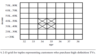
Clustering the association rules: The strong association rules obtained in the previous step are then mapped to a 2-D grid. Figure shows a 2-D grid for 2-D quantitative association rules predicting the condition buys(X, “HDTV”) on the rule right-hand side, given the quantitative attributes age and income. The four Xs correspond to the rules