Noisy Data

Introduction: Noise is a random error or variance in a measured variable. Given a numerical attribute such as, say, price, how can we “smooth” out the data to remove the noise.

Let’s look at the following data smoothing techniques:

Sorted data for price (in dollars):4, 8, 15, 21, 21, 24, 25, 28, 34

Partition into (equal-frequency) bins:

Bin 1: 4, 8, 15

Bin 2: 21, 21, 24

Bin 3: 25, 28, 34

Smoothing by bin means:

Bin 1: 9, 9, 9

Bin 2: 22, 22, 22

Bin 3: 29, 29, 29

Smoothing by bin boundaries:

Bin 1: 4, 4, 15

Bin 2: 21, 21, 24

Bin 3: 25, 25, 34

1. Binning: Binning methods smooth a sorted data value by consulting its “neighborhood,” that is, the values around it. The sorted values are distributed into a number of “buckets,” or bins. Because binning methods consult the neighborhood of values, they perform local smoothing. Figure 2.11 illustrates some binning techniques. In this example, the data for price are first sorted and then partitioned into equal-frequency bins of size 3 (i.e., each bin contains three values). In smoothing by bin means, each value in a bin is replaced by the mean value of the bin. For example, the mean of the values 4, 8, and 15 in Bin 1 is 9. Therefore, each original value in this bin is replaced by the value 9. Similarly, smoothing by bin medians can be employed, in which each bin value is replaced by the bin median. In smoothing by bin boundaries, the minimum and maximum values in a given bin are identified as the bin boundaries. Each bin value is then replaced by the closest boundary value. In general, the larger the width, the greater the effect of the smoothing. Alternatively, bins may be equal-width, where the interval range of values in each bin is constant. Binning is also used as a discretization technique and is further discussed in Section 2.6.
2. Regression: Data can be smoothed by fitting the data to a function, such as with regression. Linear regression involves finding the “best” line to fit two attributes (or variables), so that one attribute can be used to predict the other. Multiple linear regressions is an extension of linear regression, where more than two attributes are involved and the data are fit to a multidimensional surface. Regression is further described in Section 2.5.4, as well as in Chapter 6.
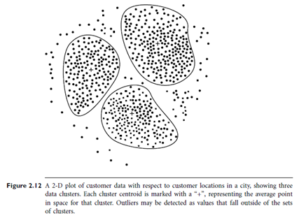
3. Clustering: Outliers may be detected by clustering, where similar values are organized into groups, or “clusters.” Intuitively, values that fall outside of the set of clusters may be considered outliers (Figure 2.12).

Many methods for data smoothing are also methods for data reduction involving discretization. For example, the binning techniques described above reduce the number of distinct values per attribute. This acts as a form of data reduction for logic-based data mining methods, such as decision tree induction, which repeatedly make value comparisons on sorted data. Concept hierarchies are a form of data discretization that can also be used for data smoothing. A concept hierarchy for price, for example, may map real price values into inexpensive, moderately priced, and expensive, thereby reducing the number of data values to be handled by the mining process. Some methods of classification, such as neural networks, have built-in data smoothing mechanisms.