Finding The Convex Hull

Finding the convex hull: The convex hull of a set Q of points is the smallest convex polygon P for which each point in Q is either on the boundary of P or in its interior. We denote the convex hull of Q by CH(Q). Intuitively, we can think of each point in Q as being a nail sticking out from a board. The convex hull is then the shape formed by a tight rubber band that surrounds all the nails. Figure 33.6 shows a set of points and its convex hull.

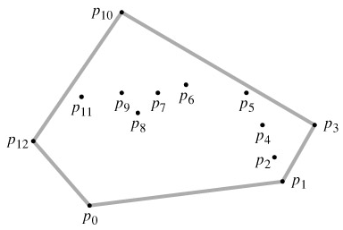
Figure 33.6: A set of points Q = {p₀, p₁, ..., p₁₂} with its convex hull CH(Q) in gray.

In this section, we shall present two algorithms that compute the convex hull of a set of n points. Both algorithms output the vertices of the convex hull in counterclockwise order. The first, known as Graham's scan, runs in O(n lg n) time. The second, called Jarvis's march, runs in O(nh) time, where h is the number of vertices of the convex hull. As can be seen from Figure 33.6, every vertex of CH(Q) is a point in Q. Both algorithms exploit this property, deciding which vertices in Q to keep as vertices of the convex hull and which vertices in Q to throw out.

There are, in fact, several methods that compute convex hulls in O(n lg n) time. Both Graham's scan and Jarvis's march use a technique called "rotational sweep," processing vertices in the order of the polar angles they form with a reference vertex. Other methods include the following.

• In the incremental method, the points are sorted from left to right, yielding a sequence 〈p₁, p₂, ..., p_n〉. At the ith stage, the convex hull of the i - 1 leftmost points, CH({p₁, p₂, ..., p_i-1}), is updated according to the ith point from the left, thus forming CH({p₁, p₂, ..., p_i}).

• In the divide-and-conquer method, in Θ(n) time the set of n points is divided into two subsets, one containing the leftmost ⌈n/2⌉ points and one containing the rightmost ⌊n/2⌋ points, the convex hulls of the subsets are computed recursively, and then a clever method is used to combine the hulls in O(n) time. The running time is described by the familiar recurrence T(n) = 2T(n/2) O(n), and so the divide-and-conquer method runs in O(n lg n) time.

• The prune-and-search method is similar to the worst-case linear-time median algorithm. It finds the upper portion (or "upper chain") of the convex hull by repeatedly throwing out a constant fraction of the remaining points until only the upper chain of the convex hull remains. It then does the same for the lower chain. This method is asymptotically the fastest: if the convex hull contains h vertices, it runs in only O(n lg h) time.

Computing the convex hull of a set of points is an interesting problem in its own right. Moreover, algorithms for some other computational-geometry problems start by computing a convex hull. Consider, for example, the two-dimensional farthest-pair problem: we are given a set of n points in the plane and wish to find the two points whose distance from each other is maximum. Although we won't prove it here, the farthest pair of vertices of an n-vertex convex polygon can be found in O(n) time. Thus, by computing the convex hull of the n input points in O(n lg n) time and then finding the farthest pair of the resulting convex-polygon vertices, we can find the farthest pair of points in any set of n points in O(n lg n) time.

		GRAHAM-SCAN(Q)
 1  let p0 be the point in Q with the minimum y-coordinate,
             or the leftmost such point in case of a tie
 2  let 〈p1, p2, ..., pm〉 be the remaining points in Q,
             sorted by polar angle in counterclockwise order around p0
             (if more than one point has the same angle, remove all but
             the one that is farthest from p0)
 3  PUSH(p0, S)
 4  PUSH(p1, S)
 5  PUSH(p2, S)
 6  for i ← 3 to m
 7       do while the angle formed by points NEXT-TO-TOP(S), TOP(S),
                     and pi makes a nonleft turn
 8              do POP(S)
 9          PUSH(pi, S)
10  return S